Table of contents
An overview 
Ions and ion switching 
Animal cell membranes send signals via electric impulses. Touch, Taste, Breath, all are encoded as impulses for the brain to interpret. Ions are molecules with a charge. As a law, energy flows through a gradient. There are two types of gradients established in this system which relays information from one part of the body to another. The first is the chemical (ion) gradient which consists of different ions in different concentrations. The second is an electrical gradient which has a net imbalance of charges. Let free, energy flows and an equilibrium is reached where the gradient ceases. The cell membrane barricades the ions and prevents the attainment of equilibria. There are pores in the cell membrane which contains channels / gates to allow the ions through. These channels are activated when certain conditions are met – like, touch. When a channel opens ions flow to minimize the electrochemical gradient. This is recorded as an impulse – a signal – which is then transmitted to the brain. For this impulse to be generated a certain threshold must be crossed. Once the signal is passed, the membrane “pumps” the unwanted ions back to reestablish the gradient.
Many diseases, including cancer, are believed to have a contributing factor in common. Ion channels are pore-forming proteins present in animals and plants. They encode learning and memory, help fight infections, enable pain signals, and stimulate muscle contraction. If scientists could better study ion channels, which may be possible with the aid of machine learning, it could have a far-reaching impact.
Technology to analyze electrical data in cells has not changed significantly over the past 20 years. If we better understand ion channel activity, the research could impact many areas related to cell health and migration. From human diseases to how climate change affects plants, faster detection of ion channels could greatly accelerate solutions to major world problems.
Data 
The data at hand is a simulated form of ion channel activity. This is a time series data, with the target to predict the number of open channels at any given time. The only features available are the time and the signal strength at that time. The data is simulated and injected with real world noise to emulate what scientists observe in laboratory experiments. There is also drift added to the data. Drift is time accumulated error resulting in horizontal signals getting skewed.
While the time series appears continuous, the data is from discrete batches of 50 seconds long 10 kHz samples (500,000 rows per batch). In other words, the data from 0.0001 - 50.0000 is a different batch than 50.0001 - 100.0000, and thus discontinuous between 50.0000 and 50.0001
Task 
In this Kaggle competition the challenge is to predict the number of open channels given the signal strength at any time. The number of open channels vary from 0, i.e, closed to 10 which makes a total of 11 classes.
This is a classification task. As a classification task, the challenge will be to predict the number of open channels from a range of open channels, i.e., from 0 to 10. This is evident in the metric used, which is the macro $f1$ score. $F1$ is calculated as follows:
$$\text{F1} = \frac{2 · \text{precision} · \text{recall}} {\text{precision} + \text{recall}}$$where:
$$\text{precision} = \frac{\text{TP}}{ \text{TP} + \text{FP}}$$and,
$$\text{recall} = \frac{\text{TP}}{ \text{TP} + \text{FN}}$$In ”macro” 𝐹1 a separate 𝐹1 score is calculated for each open channels value and then averaged.
EDA 
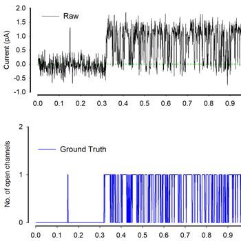
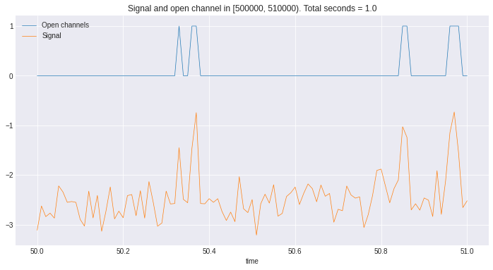
- The first thing to notice is that the signal and the open channels are linearly co-related, i.e., as the signal strength increases the number of open channels increases. Another thing to notice is that a channel only opens if the signal crosses a threshold. This knowledge can change this from a classification to a regression problem. Finding the thresholds where the signal triggers the channel to open and then using the magnitude of that signal to predict the number of open channels seems an interesting idea. The first task then, would be to align the zero of the signal to zero open channels. This makes it easier to find the threshold.
 |
|---|
| Here we see as the signal crosses the $-2ma$ threshold the channels opens up |
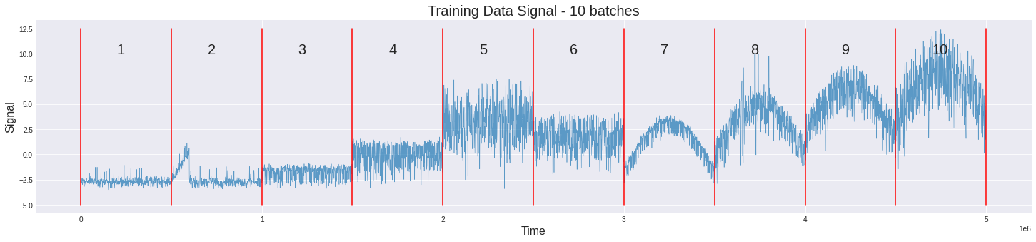
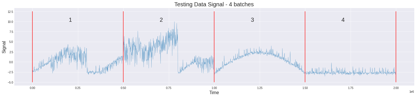
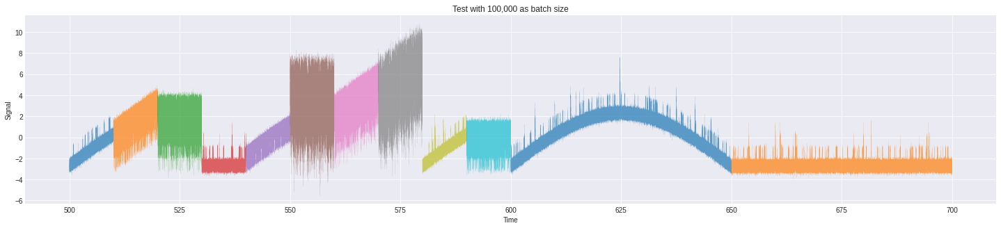
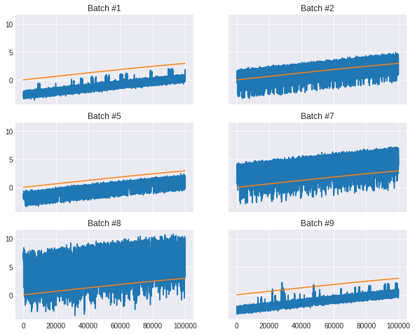
- The train data consists of 10 batches, each batch an observation made over 50$s$ at the interval of $1e-4 s$. This is given. But, this rule doesn’t fit the test data. Only the last two batches happen to observations made for 50$s$. The first two batches can be split into smaller batches of 100,000 observations. This in total makes the test have 12 batches of observation. For uniformity assuming both the test and train batches made of 100,000 observations won’t hurt. Similarity between different batches of the train and test data can be observed.
 |
|---|
| Here is an observation of the different batches in test |
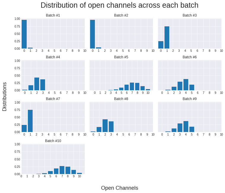
- There are mainly three types of open channels. The first is slow open, which remains closed most of the time, this is the simplest. The second type has a high rate of opening. They open very fast and make transitions very fast. The number of open channels in the second type varies from 0 to 5. The last type is the very fast open channel. These channels have a very high rate of opening. Their open channels vary from 5 to 10.
Pre-processing 
The most important task in this competition is preprocessing. Preprocessing the signal correctly makes the process of predicting open channels trivial. Since this is such a mammoth of a task, a lot of effort is expended into this.
Drift Removal 
Drift is time accumulated error resulting in horizontal signals getting skewed.There are two types of drift here:
- Linear Drift: observed as the mean signal magnitude starts increasing linearly with time
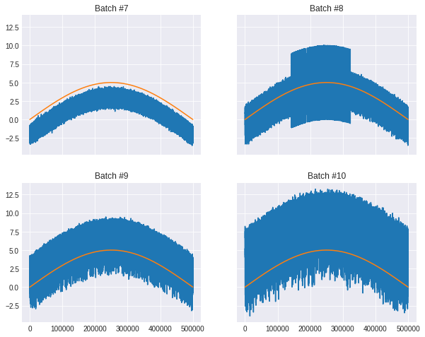
- Parabolic Drift: observed as the mean signal magnitude arches over as a parabola
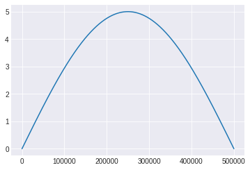
Parabolic Drift 
To remove this drift a sine function is used. A sine function of the form $\hat{y} = A sin(\omega t + \varphi) + \delta$ and $\omega = 2 \pi f$ where $f$ is the frequency of the signal, $\varphi$ is the phase of the signal and $\delta$ is a factor added to shift the origin can be used to approximate the drift. Once a good approximation for the drift is found, we simply subtract the actual signal from the value produced by the approximation to drift. The idea is to find a function such that (Given function) - (Drift function) = (Clean function)
There are three parameters to be found, namely, $A$, $\varphi$ and $\delta$. Since, each batch can have different parameters, we do this for each batch separately.
Here, the batch size is $500,000 \times 10^{-4} s$, i.e, 50$s$, and the drift is only from the first half of the sine wave. So, $\omega = \frac{2 \pi}{50 \times 2}$. We divide by 2 because the time period of half sine wave is half that of a full sine wave. We have,
$$\hat{y} = A sin(\omega x + \varphi) + \delta$$We expand $sin$ by using $sin(A + B) = sin(A)cos(B) + cos(A)sin(B)$
$$\hat{y} = Asin(\omega x)cos(\varphi) + Acos(\omega x)sin(\varphi) + \delta$$further rearranging,
$$\hat{y} = Acos(\varphi)sin(\omega x) + Asin(\varphi)cos(\omega x) + \delta$$Here, finding the three constants, namely $Acos(\varphi),\; Asin(\varphi),\;$and $\delta$, will give us an approximation to the drift function. Since we have $N = 500,000$ observations(1 batch), we need to solve a system of linear equations for which the above equation holds.
$$\begin{bmatrix}\sin(\omega x_1) & \cos(\omega x_1) & 1 \\\vdots & \vdots & \vdots \\\sin(\omega x_N) & \cos(\omega x_N) & 1\end{bmatrix}\begin{bmatrix}A\cos(\varphi) \\A\sin(\varphi) \\\delta\end{bmatrix} = \begin{bmatrix}y_1 \\ \vdots \\ y_N\end{bmatrix}$$$\mathbf{x} = (x_1, \cdots, x_N)$, is the time of observation, and $\mathbf{y} = (y_1, \cdots, y_N)$ is the signal observed at that time. In short,
$$\mathbf{M}\mathbf{\theta} = \mathbf{y}$$Here $\theta = (\theta_1, \theta_2, \theta_3)\;$ is the vector of the constants we intend to find. Notice that, $A^2 = \theta_1^2 + \theta_2^2$, as $sin^2(x) + cos^2(x) = 1$ and $\varphi = tan^{-1}(\frac{\theta_2}{\theta_1})$ as $tan(x) = \frac{sin(x)}{cos(x)}$
Once the drift function is obtained, all we have to do is to subtract it from the original signal to eliminate it
Using the above formulation we find the drift to have an amplitude of 5. The angle $\varphi$ is either $\pi$ or 0. It's $\pi$ when the index is odd and 0 otherwise. This phase difference comes because the negative part is not considered. We will use these to remove drift
 |
|---|
| sine wave used to approximate drift |
 |
|---|
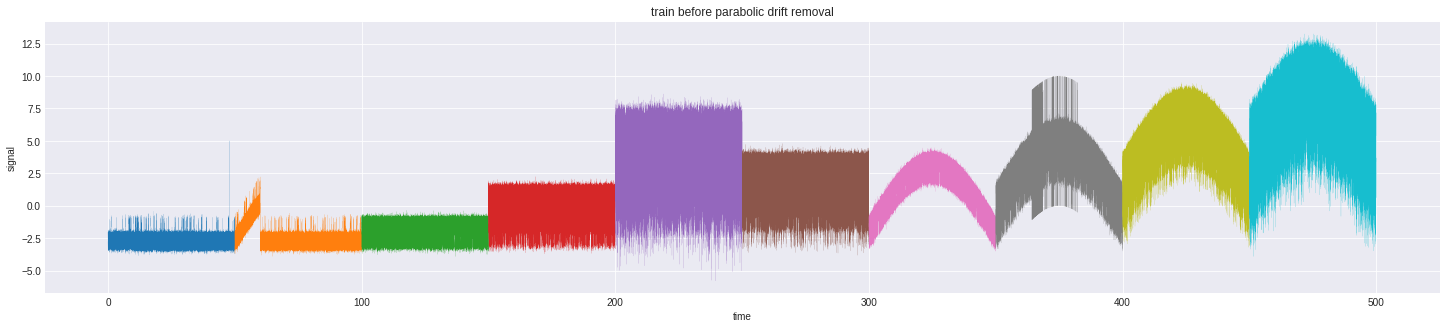
| Before removal of parabolic drift |
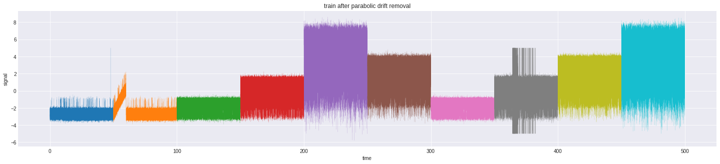 |
|---|
| After removal of parabolic drift |
Linear Drift 
The key observation to make here is that linear drift is just the first part of the parabolic drift. It then becomes easy to remove it.
Linear Transforms 
After removing drift we have semi clean data. This in itself is useful to use in a predictive model, but we preprocess it further to better our results.
Zero off set: As noted in EDA, aligning the zero of our signals to zero open channels gives us a good starting point to better predict other open channels. Here we off-set the zero of the signal with zero open channels
Scale and shift: After having the zeros aligned, we would like to align the signals with their respective open channels. We would like to also scale the signal to match the range of open channels. To do so we use linear regression. We multiply the signal with the slope obtained through linear regression and shift the signal by the regression coefficient. Since each group of the channels may have a different base shift and scale, we work with groups.
 |
|---|
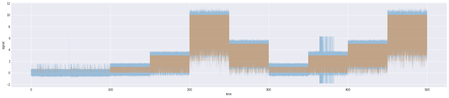
| Aligning signal with open channels |
Remove Outliers 
Outliers always pose a threat to learning. Removing outliers is quintessential in any learning process. But at the same time removing outliers leads to losing data. A nice trick to prevent this is to replace the corrupted part with corresponding open channels with added Gaussian noise. By finding the mean and standard deviation of signal minus open channels of all batches, we get the approximate noise to be added.
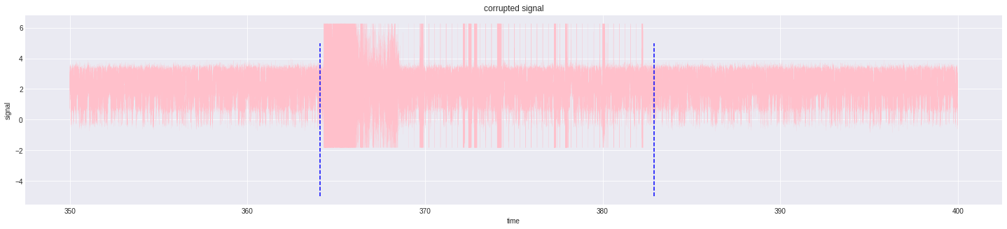 |
|---|
| outliers visualised |
Denoise 
Remove bias 
Bias is the error in our model that creeps in due to faulty assumptions about our data. Since the number of open channels is very sensitive to the signal strength, this becomes very important. We can approximate noise to be signal minus signal round. By repeatedly subtracting the mean of the noise we get a signal that's almost a round number. Because the signals are linearly transformed to fit both the scale and the off-set of open channels, a rounded signal can approximate the open channels sufficiently.
Kalman Filters 
A Kalman filter is a signal processing approach to remove Gaussian noise in the data. The Kalman filter is a state estimator that makes an estimate of some unobserved variable based on noisy measurements. It is a recursive algorithm as it takes the history of measurements into account.
The idea behind Kalman filter is this: The observation made at time $t$, is dependent on a hidden state at that time and has some inherent Gaussian noise. The hidden state depends on the state at time $t-1$, a transition rate and an inherent noise of the process. Put in equation,
$$\mathbf{x}(t) = A\mathbf{x}(t-1) + \mathbf{w}(t) \\ \mathbf{y}(t) = C\mathbf{x}(t) + \mathbf{v}(t)$$Here, $\mathbf{x}$, is the hidden state and $\mathbf{w}$, is the corresponding process noise. $\mathbf{y}$, is the observed value — in our case the signal — and $\mathbf{v}$ is the observation error. $A$ and $C$ are transition matrix and observation matrix respectively. The Kalman process tries to model the hidden state probabilistically using an iterative approach. It is an unsupervised learning algorithm and has update equations just like SGD. By successfully modelling the internal state, it tries to reduce observational noise.
Power line noise 
Since the observations were recorded with devices connected to the electric grid, some noise from the power line can be introduced. To remove this noise we use fast fourier transform. Complete removal might leed to loss of information and hence, only a fraction of the noise is removed. Since the power line uses 50Hz, frequencies in that range can be removed.
Feature Engineering 
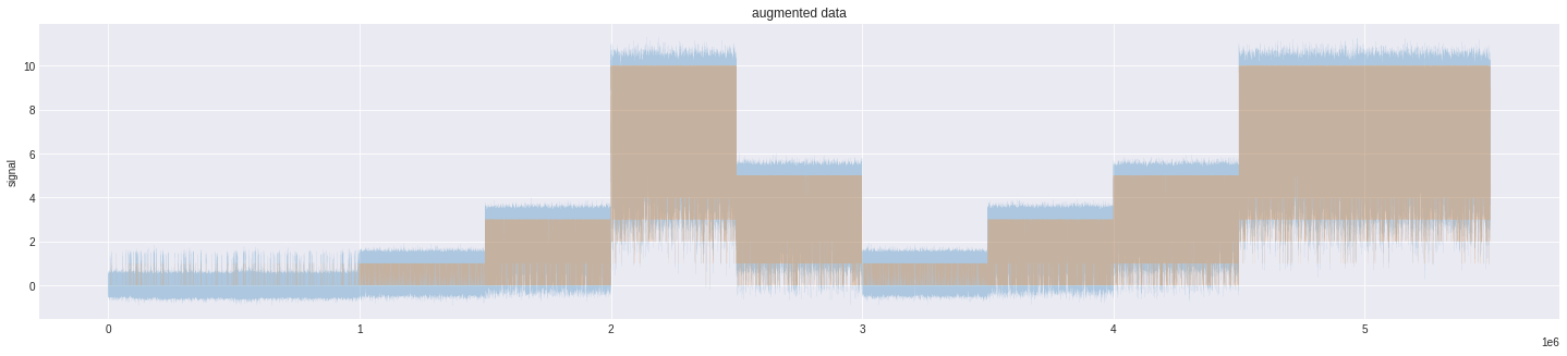
It is well understood that more data is always yield better results with any model. Here, we make a simple observation that summation of the signals from two batches are alike to the one present in the data. We can use this data as new training examples
 |
|---|
| more data created |
Since the range scale of both open channels and signal is the same, rounding the signal will be a good feature. Standard scaling each batch of the signal gives a relativistic way to check for open channels this seems a good feature. The power of a signal is proportional to the square of the signal. This can also be used as a feature. Since the process is a hidden Markov model, it depends only on the states directly preceding and directly succeeding it. If the data was a time series data considering the future would not be possible. But, since the data is a HMM, the future state is as influential as the past state. Since this is such an important feature we shift the data by steps of 1, 2, 3, 4 and 5. Calculating the percentage change between the signal and the shifted signal is also considered. Finally, we bin and encode the signal so that it can be related to the signal.
Training 
This is a highly tuned lgbm model. Tuning is done using optuna. This is the best single model. The lgbm out of fold probabilities are saved to be blended in with other models. This receives a cross validation score of 0.9401.
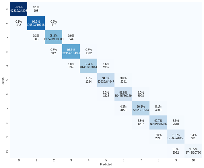
One can see from the confusion matrix that it becomes harder to classify as the number of open channels increase
An ExtraTreesRegressor was trained to:
- demonstrate how regression can be used in this setting
- Add variety to the blend
Wavenet was the final ensemble. It was the blend of all the 7 (6 lgbm classifiers and 1 extra trees regressor) previous model. Wave net was large enough to not fit in GPU memory, and so the training was done in groups of 5000 training samples. To further increase the score the data set was augmented by flipping and stacking. Test time augmentation was also explored.
def augment(X, y):
    '''
    augments the data by flipping and appending to the existing data
    '''
    X = np.vstack((X, np.flip(X, axis=1)))
    y = np.vstack((y, np.flip(y, axis=1)))

    return X, y
The most important part of wavenet is the waveblock which consists of dilated convolutions. Dilated Convolutions are a type of convolution that “inflate” the kernel by inserting holes between the kernel elements. An additional parameter $l$, (dilation rate) indicates how much the kernel is widened. There are usually $l-1$, spaces inserted between kernel elements. The normal convolutions are just have $l = 1$. Dilated convolution is a way of increasing receptive view of the network exponentially while still maintaining linear parameter growth, i.e., It captures more contextual information with less parameters giving a border view at the cost of neglecting detail.
 |
|---|
| This animation shows how a WaveNet is structured. It is a fully convolutional neural network, where the convolutional layers have various dilation factors that allow its receptive field to grow exponentially with depth and cover thousands of timesteps. |
Future Work 
Due to time constraints only lgbm and wavenet were explored. Exploring more different models and different ensemble techniqus would have resulted in a better score. Some models like GRU, Conv1D, and even simple MLP's could be tried.
Since the process is known to be a HMM, more efforts can be expended on discovering better HMM models. Factorial HMM's seem very promising. Since HMM's are robust to outliers and to noise, research into them will be very fruitful. Better preprocessing and better signal processing may yield even better results with the already used models.